Hessian Matrix
In mathematics, the Hessian matrix or Hessian is a square matrix of second-order partial derivatives of a function. It describes the local curvature of a function of many variables. The Hessian matrix was developed in the 19th century by the German mathematician Ludwig Otto Hesse and later named after him. Hesse originally used the term "functional determinants".
Given the real-valued function
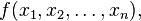
if all second partial derivatives of f exist and are continuous over the domain of the function, then the Hessian matrix of f is
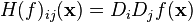
where x = (x1, x2, ..., xn) and Di is the differentiation operator with respect to the ith argument. Thus
![H(f) = \begin{bmatrix}
\dfrac{\partial^2 f}{\partial x_1^2} & \dfrac{\partial^2 f}{\partial x_1\,\partial x_2} & \cdots & \dfrac{\partial^2 f}{\partial x_1\,\partial x_n} \\[2.2ex]
\dfrac{\partial^2 f}{\partial x_2\,\partial x_1} & \dfrac{\partial^2 f}{\partial x_2^2} & \cdots & \dfrac{\partial^2 f}{\partial x_2\,\partial x_n} \\[2.2ex]
\vdots & \vdots & \ddots & \vdots \\[2.2ex]
\dfrac{\partial^2 f}{\partial x_n\,\partial x_1} & \dfrac{\partial^2 f}{\partial x_n\,\partial x_2} & \cdots & \dfrac{\partial^2 f}{\partial x_n^2}
\end{bmatrix}.](http://upload.wikimedia.org/math/f/7/2/f7296865484b39fcbac598a99b7f3dbb.png)
Because f is often clear from context,  is frequently abbreviated to
  .
.
is frequently abbreviated to . .
.
The determinant of the above matrix is also sometimes referred to as the Hessian.[1]
Hessian matrices are used in large-scale optimization problems within Newton-type methods because they are the coefficient of the quadratic term of a local Taylor expansion of a function. That is,

where J is the Jacobian matrix, which is a vector (the gradient) for scalar-valued functions. The full Hessian matrix can be difficult to compute in practice; in such situations, quasi-Newton algorithms have been developed that use approximations to the Hessian. The best-known quasi-Newton algorithm is the BFGS algorithm
Jacobian Matrix
In vector calculus, the Jacobian matrix is the matrix of all first-order partial derivatives of a vector-valued function. Specifically, suppose  is a function (which takes as input real n-tuples and produces as output real m-tuples). Such a function is given by m real-valued component functions,
  . The partial derivatives of all these functions with respect to the variables
  (if they exist) can be organized in an m-by-n matrix, the Jacobian matrix
  of
of  , as follows:
is a function (which takes as input real n-tuples and produces as output real m-tuples). Such a function is given by m real-valued component functions, . The partial derivatives of all these functions with respect to the variables (if they exist) can be organized in an m-by-n matrix, the Jacobian matrix of , as follows: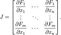
No comments:
Post a Comment