2013-3-2
OpenOF Framework for Sparse Non-linear Least Squares Optimization on a GPU
With OpenOF, a framework is presented, which enables developers to design
sparse optimizations regarding parameters and measurements and utilize the
parallel power of a GPU
This
code is written in Python with three major libraries: Thrust, CUSP and SymPy. Code framework is written in Python but can also generate C++ code.
Code website
https://github.com/OpenOF/OpenOF
Process of Nonlinear least squares optimization:
1. Iterative method
2. Linearize the cost function in each iteration
3. Levenberg-Marquardt(LM) algorithm is standard, combing the Gauss-Newton algorithm with the gradient descent approach. LM guarantees convergence.
4. In each interation , solving linear
Ax = b is most intensive.
5. Sparse matrix representation is used:
sparseLM (Lourakis, 2010) and
g2o (Kummerle et al., 2011), but on CPU
6. Solving
Ax =b, many algorithms can achieve,
Cholesky docomposition A = LDL'
7. this paper use
Conjugate gradient (CG) approach on GPU.
Nonlinear least squares optimization is widely used in SLAM and BA.
The authors' some comments about three BA libraries:
1.The
SBA library (Lourakis and Argyros,2009) takes advantage of the special structure of the
Hessian matrix to apply the
Schur complement for solving the linear system. Nevertheless it has several drawbacks. Integrating additional parameters which remain identical for all measurements (e.g. camera calibration) is not possible, as the structure would change such that the Schur complement could not be applied anymore.
2. sparseLM (Lourakis, 2010) is slow.
3. g2o: the Jacobian is evaluated by numerical differentiation which is time consuming and also degrades the convergence rate.
4. ISAM: (Kaess et al., 2011),which address only
a subset of problems, have been presented previously for least squares optimization
Overall Comment: this paper is claims to present an open source framework for sparse nonlinear opitmization. The cost functions is described in high level scripting language. It can not be used without GPU yet. It seems for me g2o or iSam would be more useful on CPU.


 .
.![(k_1, k_2, p_1, p_2[, k_3[, k_4, k_5, k_6]])](http://docs.opencv.org/_images/math/7c67b59b59778bc682b2d972bde3d910b2326924.png) of 4, 5, or 8 elements. If the vector is NULL/empty, the zero distortion coefficients are assumed.
of 4, 5, or 8 elements. If the vector is NULL/empty, the zero distortion coefficients are assumed.


![[t,t+T]](https://upload.wikimedia.org/math/6/4/8/648573482abe10af9ae83915e5751af8.png)

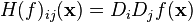
![H(f) = \begin{bmatrix}
\dfrac{\partial^2 f}{\partial x_1^2} & \dfrac{\partial^2 f}{\partial x_1\,\partial x_2} & \cdots & \dfrac{\partial^2 f}{\partial x_1\,\partial x_n} \\[2.2ex]
\dfrac{\partial^2 f}{\partial x_2\,\partial x_1} & \dfrac{\partial^2 f}{\partial x_2^2} & \cdots & \dfrac{\partial^2 f}{\partial x_2\,\partial x_n} \\[2.2ex]
\vdots & \vdots & \ddots & \vdots \\[2.2ex]
\dfrac{\partial^2 f}{\partial x_n\,\partial x_1} & \dfrac{\partial^2 f}{\partial x_n\,\partial x_2} & \cdots & \dfrac{\partial^2 f}{\partial x_n^2}
\end{bmatrix}.](http://upload.wikimedia.org/math/f/7/2/f7296865484b39fcbac598a99b7f3dbb.png)
 is frequently abbreviated to
  .
. .
.
 is a function (which takes as input
  . The partial derivatives of all these functions with respect to the variables
  (if they exist) can be organized in an m-by-n matrix, the Jacobian matrix
  of
of  , as follows:
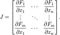

 factorization; the matrix
  are solved instead of the original system
  .
.


